
 In my first post on inferential statistics, I wrote about defining a population and constructing a random sample based on a hypothetical scenario that’s typical of some projects that we at KCIC encounter in our Consulting work. In the example, I described a time KCIC was tasked with reliably confirming that invoice summary information contained in spreadsheet form was in fact supported by hard copy evidence. My first post explained my construction of a random sample from a given population, in this case, all of the individual dollars. In my second post, I listed some important considerations when choosing a sample size – and the impact of those choices on the final analysis. Today, I want to focus on how to construct a confidence interval and why it is critical for extrapolating conclusions.
Determining Sample Size
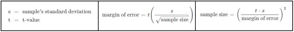
Unless statistics is your “thing,” this calculation can feel complicated. To simplify – let me break down the formulas (below) using nice, round numbers. Hypothetically, let’s say the spreadsheet has $100 million total on 1,000 separate invoices. Given time and resource constraints, we decide that the most we can review is 100 invoices, which becomes our sample size. Two variables remain: standard deviation and t-value.
Finding Standard Deviation
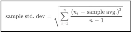
The standard deviation is a measurement that illustrates how close individual observations are to the mean. Below is the formula with “n” equal to the number of items in the sample (sample size).
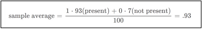
After reviewing our 100-invoice dollar sample, we find that 93 of the dollars have hard copy invoice evidence to back them up. We can calculate the sample’s average by creating a true or false statement and assigning true as equal to a value of 1 and false as equal to a value of 0. Our statement is that invoice evidence is present. Therefore, if invoice evidence is present for a reviewed dollar, then we assign a value of 1 and if it is missing, then we assign a value of 0. We calculate the sample average to be .93:
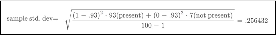
Using the formula for sample standard deviation, we find the sample’s standard deviation to be 0.256432:
Finding t-value
All we need to do for the t-value is look it up! The t-value is found on a standard t-table. If we want to use a 99% confidence level, then for a sample size of 100, the corresponding t-value is 2.364.
Calculating Margin of Error
Finally, we can apply these three variables to the equation to find the margin of error. That gives us a result of 6.06 percent:

Constructing a Confidence Interval
The confidence interval is the range bounded by the average sample value (93%) minus the margin of error (lower bound) and the average sample value plus the margin of error (upper bound). This means that our confidence interval is between 86.94% and 99.06%.
Interpreting Results
So we have completed the random sample and calculated the resulting confidence interval based on a 99% level of confidence … but what does it all mean? And just as importantly, what does it not mean?
Since we used a 99% confidence level, we can say that 99 times out of 100, we expect that in the summary, the number of dollars with hard copy invoice evidence will be between 86.94% and 99.06% of the population’s total invoice dollars ($100 million), or in this case between $86.94 million and $99.06 million. This does not mean that the population’s total is without a doubt within this range. We could find it to be higher or lower if we reviewed every invoice. However, given the time and resources available, we can make a very confident statistical inference and use it as a basis for KCIC expert testimony or as information to help our client make time-sensitive decisions.